

Positive Line On A Graph
Quickly create a positive negative bar nautical chart in Excel
If you want to show how multiple units does comparison to each other based on the same criteria conspicuously, you tin use the positive negative bar chart which can display positive and negative development very skillful as beneath screenshot shown.
3 steps to create a positive negative nautical chart in Excel |
| Here are dozens of chart tools in Kutools for Excel which can help you lot generate some circuitous charts quickly. 1 of them is Positive Negative Bar Nautical chart, it can create a beautiful and editable chart for yous in 3 steps. Click to free download this tool. |
 |
Create positive negative bar chart stride by step (15 steps)
Arraneg data
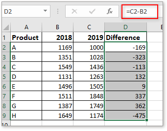
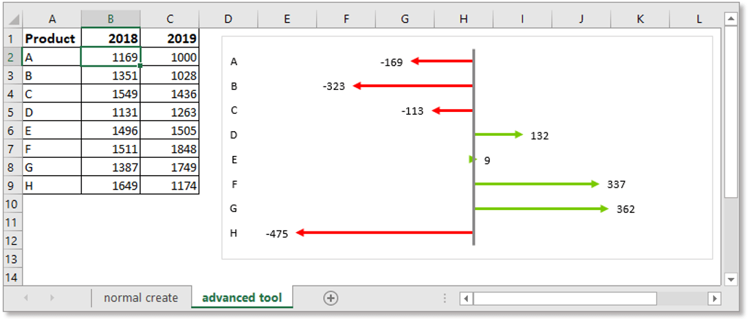
Supposing the original information displayed as below:

Firstly, add some helper columns:
1. Calculate the difference between two columns (Cavalcade C and Cavalcade B)
In cell D2, type this formula
=C2-B2
Drag fill handle down to calculate the differences.
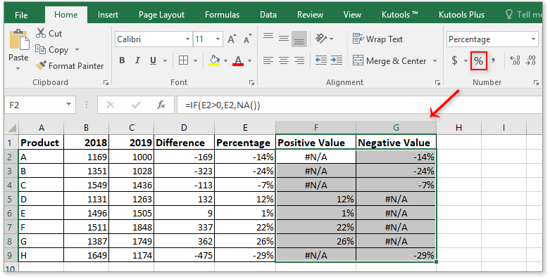
two. Calculate the increase or decrease pct
In cell E2, blazon this formula
=D2/B2
Drag make full handle down to fill up cells with this formula

So keep cells selected, click Abode tab, and become to the Number group, choose Percent Style button to format the cells shown as percentage.

3. Calculate the positive value and negative value
In cell F2, type this formula
=IF(E2>0,E2,NA())
E2 is the percentage cell, drag fill handle down to fill the cells with this formula.

In Cell G2, blazon this formula
=IF(E2<0,E2,NA())
E2 is the percentage cell, drag make full handle down to fill the cells with this formula.

Now, select F2: G9, click Home > Percentage Mode to format these cells as percentages.
Create chart
Now create the positive negative bar chart based on the data.
1. Select a blank cell, and click Insert > Insert Column or Bar Chart > Clustered Bar.

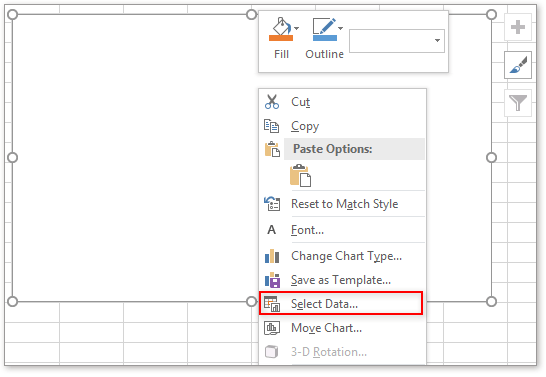
2. Right click at the blank chart, in the context carte du jour, cull Select Information.
three. In the Select Data Source dialog, click Add together button to open up the Edit Series dialog. In the Series proper noun textbox, choose the Percentage header, then in the Serial values textbox, cull E2:E9 that contains increasing and decreasing percentages, click OK.
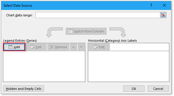

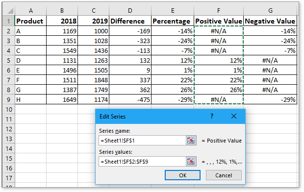
iv. Back to the Select Data Source dialog, click Add to go to the Edit Serial dialog again, select F1 as the series name, and F2:F9 equally the series values. F2:F9 are the positive values, Click OK.
5. Again, Click Add in the Select Data Source dialog to go to the Edit Series dialog, select G1 every bit series name, G2:G9 equally series values. Click OK.

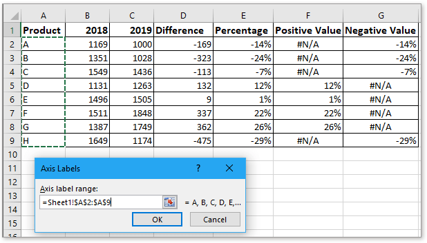
six. Dorsum to the Select Information Series dialog, click Edit button in the Horizontal (Category) Axis Labels section, and choose A2:A9 as the axis label names in the Axis Labels dialog, click OK > OK to cease the select data.

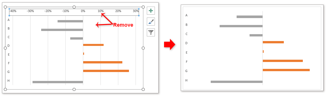
Now the chart is displayed every bit below:
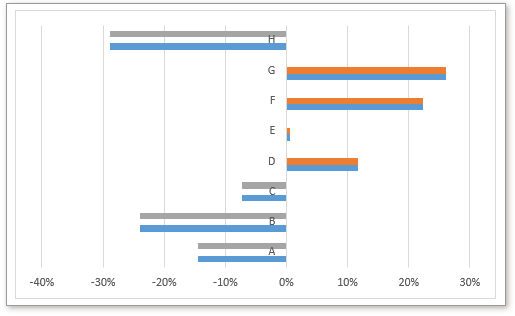
Then select the blue series, which express the increasing and decreasing per centum values, click Delete to remove them.
Arrange chart
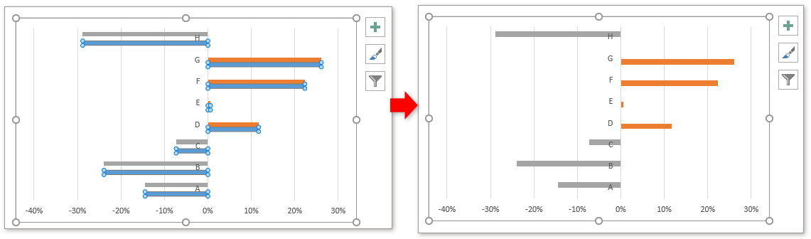
Then accommodate the chart.
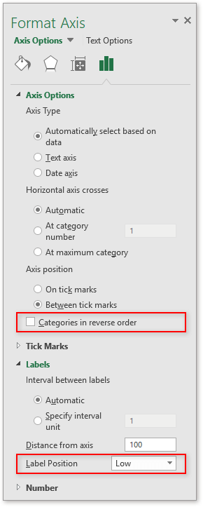
ane. Right click at the centrality labels, so choose Format Axis from context menu, and in the popped Format Axis pane, check Categories in reverse order checkbox in Axis Options department, and scroll downward to the Labels section, cull Low from the drop-down list beside Label Position.

2. Remove gridlines and X (horizontal) axis.
3. Right click at i series to select Format Data Point from the context carte, and in the Format Data Point pane, accommodate Series Overlap to 0%, Gap Width to 25%.

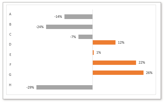
4. Right click at left series, and click Add together Data Label > Add Data Labels.


5. Remove the #N/A labels one by one.
six. Select the chart to show the Design tab, and under Design tab, click Add together Nautical chart Element > Gridlines > Main Major Horizontal.

You tin modify the series color and add chart title as you lot need.
This normal way tin create the positive negative bar chart, but it is troublesome and takes much fourth dimension. For users who want to quickly and hands handle this chore, you lot can endeavor beneath method.
Create positive negative bar chart with a handy tool (iii steps)
With the Positive Negative Bar Chart tool of Kutools for Excel, which merely needs 3 steps to deal with this job in Excel.
one. Click Kutools > Charts > Positive Negative Bar Chart.

2. In the popping dialog, choose ane chart blazon you lot need, the choose the centrality labels, two serial values separately. So click Ok.

3. And then a dialog pops out to remind you it volition create a new sheet to store some data, if y'all want to continue create the chart, click Yes.

Now a positive negative chart has been created, at the aforementioned time, a hidden canvas created to place the calculated data.
Type 1

Type two
Yous can format the generated nautical chart in Pattern and Format tab every bit yous demand.
Sample file
Click to download sample file
Other Operations (Articles)
How to create thermometer goal chart in Excel?
Have y'all always imaged to create a thermometer goal chart in Excel? This tutorial will bear witness you the detailed steps of creating a thermometer goal nautical chart in Excel.
Alter chart color based on value in Excel
Sometimes, when you insert a nautical chart, y'all may want to prove different value ranges as unlike colors in the nautical chart. For case, when serial value (Y value in our example) in the value range 10-30, prove the series color as ruby; when in value range 30-50, evidence color as dark-green; and when in value range fifty-70, bear witness colour as purple. Now this tutorial will introduce the way for you to alter chart color based on value in Excel.
Create an interactive chart with serial-selection checkbox in Excel
In Excel, nosotros ordinarily insert a chart for ameliorate displaying information, sometimes, the chart with more than than ane series selections. In this case, y'all may want to show the serial past checking the checkboxes. Supposing there are ii series in the chart, check checkbox1 to display series ane, check checkbox2 to display series 2, and both checked, display ii series
The Best Office Productivity Tools
Kutools for Excel Solves Almost of Your Problems, and Increases Your Productivity by 80%
- Super Formula Bar (easily edit multiple lines of text and formula); Reading Layout (easily read and edit big numbers of cells); Paste to Filtered Range...
- Merge Cells/Rows/Columns and Keeping Data; Split Cells Content; Combine Duplicate Rows and Sum/Average... Prevent Duplicate Cells; Compare Ranges...
- Select Indistinguishable or Unique Rows; Select Blank Rows (all cells are empty); Super Find and Fuzzy Detect in Many Workbooks; Random Select...
- Exact Copy Multiple Cells without changing formula reference; Automobile Create References to Multiple Sheets; Insert Bullets, Bank check Boxes and more than...
- Favorite and Chop-chop Insert Formulas, Ranges, Charts and Pictures; Encrypt Cells with password; Create Mailing List and send emails...
- Excerpt Text, Add together Text, Remove past Position, Remove Space; Create and Impress Paging Subtotals; Catechumen Betwixt Cells Content and Comments...
- Super Filter (salvage and apply filter schemes to other sheets); Advanced Sort by month/week/solar day, frequency and more; Special Filter by bold, italic...
- Combine Workbooks and WorkSheets; Merge Tables based on key columns; Divide Data into Multiple Sheets; Batch Convert xls, xlsx and PDF...
- Pivot Table Grouping past week number, day of week and more than... Evidence Unlocked, Locked Cells past dissimilar colors; Highlight Cells That Have Formula/Name...
")
Office Tab - brings tabbed interface to Function, and make your work much easier
- Enable tabbed editing and reading in Word, Excel, PowerPoint , Publisher, Access, Visio and Project.
- Open and create multiple documents in new tabs of the same window, rather than in new windows.
- Increases your productivity by 50%, and reduces hundreds of mouse clicks for you every 24-hour interval!
")

Positive Line On A Graph,
Source: https://www.extendoffice.com/documents/excel/5960-excel-positive-negative-bar-chart.html
Posted by: blairgual1950.blogspot.com
0 Response to "Positive Line On A Graph"
Post a Comment